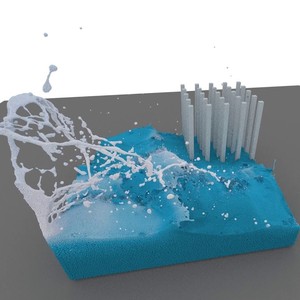
Neural Operator

Is data all you need to model the world? An insight into the paradigm of data-driven scientific ML

IEEE Transactions on Pattern Analysis and Machine Intelligence (TPAMI), 2026

Hrishikesh Viswanath^1* Md Ashiqur Rahman¹ Abhijeet Vyas¹ Andrey Shor¹ Beatriz Medeiros² Stephanie Hernandez Suhas Eswarappa Prameela³ Aniket Bera¹

¹Department of Computer Science, Purdue University, West Lafayette, IN, USA ²Department of Engineering, University of Cambridge, Cambridge, United Kingdom
³Department of Materials Science and Engineering, Department of Metallurgical Engineering and Department of Mechanical Engineering, University of Utah, UT, USA
^*Corresponding author

Paper (IEEE) BibTeX

TL;DR

A survey of neural operators: data-driven models that learn mappings between function spaces and offer a fast, discretization-invariant complement to conventional PDE solvers such as finite elements and finite differences. It covers how these models can help solve physics and engineering problems, and the open problems that machine-learning approaches still face.

Scope of the Survey

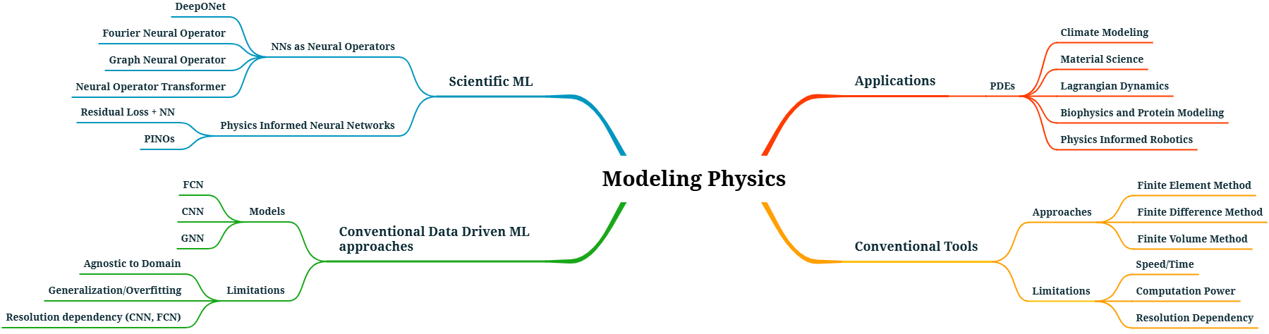
Flowchart of conventional and ML-based approaches to solving PDEs — The logical flow of how PDEs can be solved using various methods, highlighting existing ML techniques and the families of neural operator-based techniques.

The survey covers data-driven and physics-informed neural operators within the broader realm of scientific ML. It evaluates these models along three axes (scalability, generalizability, and sensitivity to training data quality) and discusses the open problems in each. It then reviews benchmark datasets and controlled settings, and three classes of applied problems: large-scale forecasting and long-range temporal problems, modeling heterogeneous systems, and inverse problems.

What Is a Neural Operator?

Instead of learning the solution to one discretized instance of a PDE, operator learning learns the map between infinite-dimensional function spaces,

$$\mathcal{G}: \mathcal{A} \to \mathcal{U}, \qquad \text{trained on pairs } \{a_i, u_i\}_{i=1}^{N}.$$

Its defining property is discretization invariance: a model trained at one resolution can be evaluated at any other. This enables rapid inference, orders of magnitude faster than classical solvers, and mesh independence, for example training on a $40 \times 40$ grid and evaluating on $256 \times 256$ without retraining ("zero-shot super-resolution").

Taxonomy of architectures

The field originated with two paradigms. Branch–trunk architectures (DeepONet) encode the input function and the query coordinates with two sub-networks and take their dot product. Integral kernel architectures iterate the transformation

$$(K_a u)(x) = \int_D \kappa\big(x, y, a(x), a(y)\big)\, u(y)\, dy,$$

approximated by message passing on graphs (GNO) or as a multiplication in Fourier space after an FFT, truncated at $k_{max}$ modes (FNO). Task-specific variants followed: geometry-aware operators for irregular domains (Geo-FNO, GINO); transformer and generative backbones (AFNO, IPOT, GNOT, Transolver; GANO, DSNO); physics-informed neural operators that add a PDE residual to regularize the operator (PINO); multiwavelet operators for localized high-frequency features (MWNO); and foundation-style pre-trained and modular frameworks (CoDANO, UPT).

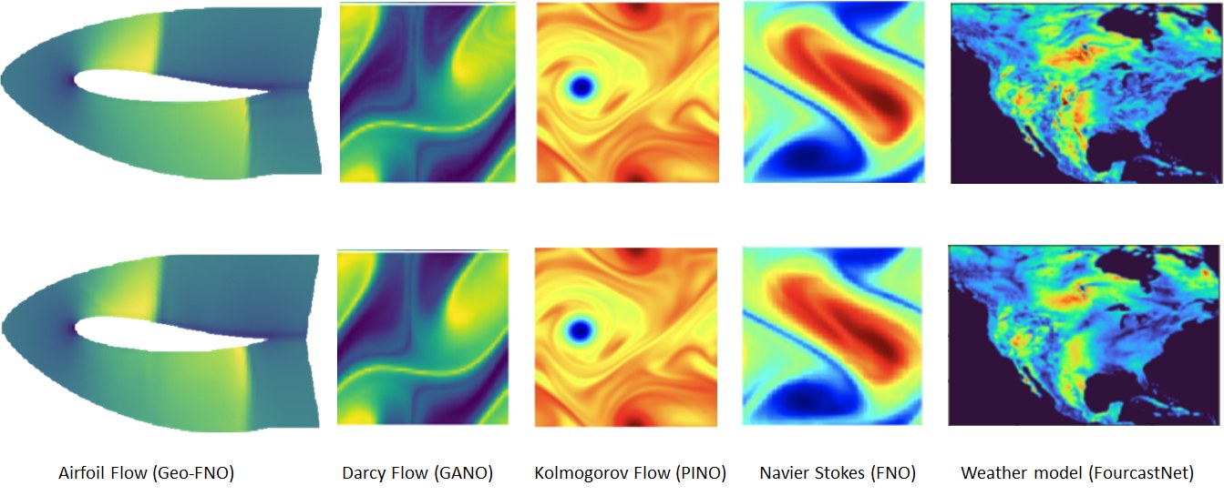
Ground truth vs. neural operator predictions on five problems — Ground truth (top) vs. operator predictions (bottom): airfoil flow by Geo-FNO (Liu et al.), Darcy flow by GANO (Rahman et al.), Kolmogorov flow by PINO (Li et al.), Navier–Stokes by FNO (Li et al.), and weather forecasting by FourCastNet (Pathak et al.).

Seminal architectures at a glance

Model	Advantages	Limitations
Fourier neural operator	Faster; resolution and discretization invariant; data driven; doesn't need to know the underlying PDE; zero-shot super-resolution	Aliasing errors; only works on rectangular domains with uniform meshes; overfits with deeper networks
DeepONet	Approximates mappings between infinite-dimensional Banach spaces; learns oscillatory continuous functions	Requires a high amount of training data; not resolution invariant (fixed input discretization)
Graph neural operator	Learns long-range dependencies in graph-like data; linear time complexity; discretization invariant	Outperformed by FNO on all PDEs with regular meshes
PINO	Overcomes the limitations of purely physics-based and purely data-driven approaches; combines coarse- and high-resolution data	Not rigorously tested on high-dimensional PDEs
Geo-FNO	Geometry aware; accepts irregular meshes and point clouds	Only tested on regular homeomorphic topologies
Multiwavelet NO	Compact representation; resolution-independent solutions	Cannot generalize to high-frequency signals from low-frequency ones

Condensed from the survey's comparison table, which also covers GANO/UNO, Adaptive FNO, Implicit FNO and Spectral NO.

Open Problems

Neural operators are not yet a panacea. The survey organizes the challenges of moving from theoretical universality to practical deployment along three axes.

Data sensitivity & robustness

Grid sensitivity: aliasing errors when the inference grid differs significantly from the training grid.
Noise accumulation: errors compound over long auto-regressive rollouts.
Data requirements: scarce or noisy data can lead to spurious minima that violate physical laws.

Generalizability & stability

Physics-informed optimization: PDE losses can fail on high convection or stiff reaction–diffusion terms.
Geometric generalization: extrapolating to unseen, topologically distinct large-scale domains remains open.

Scalability & cost

Parameterization trade-off: larger models generalize better, at a steep training cost.
Training vs. inference: reducing the break-even point against classical solvers.
Curse of dimensionality: high-dimensional PDEs (e.g. Boltzmann) remain prohibitive.

Benchmarks

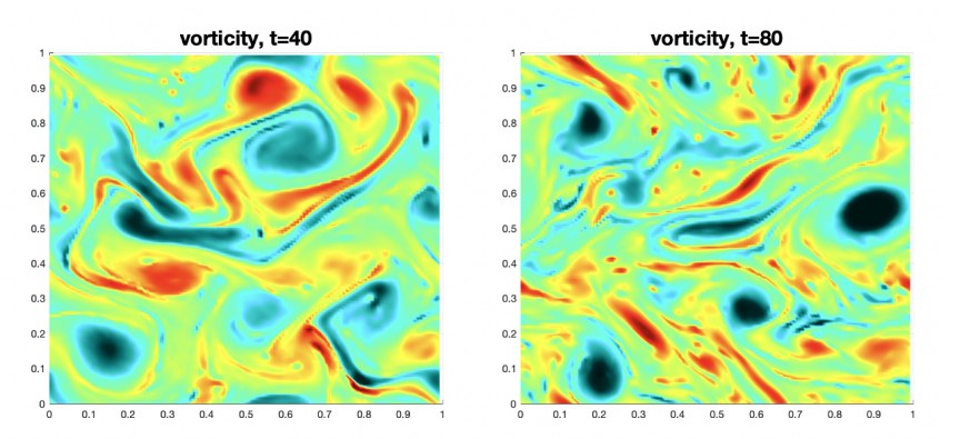
Eulerian benchmarks (Darcy flow, Poisson and heat equations, Burgers', Kolmogorov flow, Kármán vortex street) test mappings between fields; Lagrangian benchmarks test physical interactions on dynamic, unstructured graphs, bridging scientific ML and computer graphics.

Simulations from The Well — Simulating fluid flow over complex settings is a challenging task, as illustrated by The Well (Ohana et al.).

The GNS dataset (Sanchez-Gonzalez et al.): fluids and deformable materials simulated with MPM and SPH.

MeshGraphNets datasets — Eulerian, Lagrangian and mesh-based simulation datasets from MeshGraphNets (Pfaff et al.).

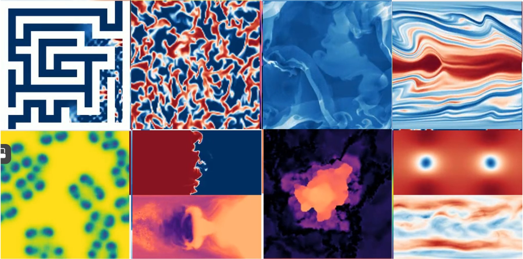
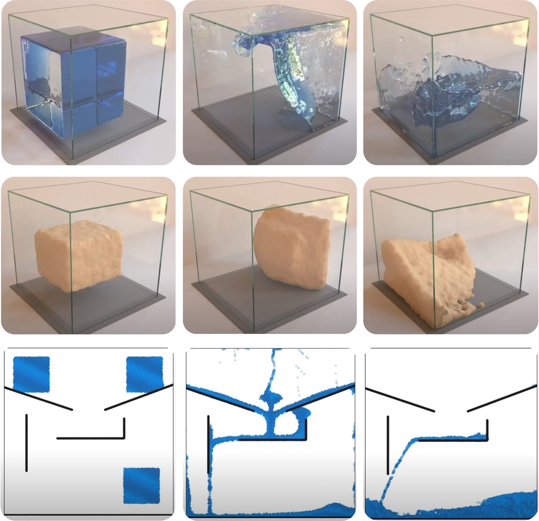
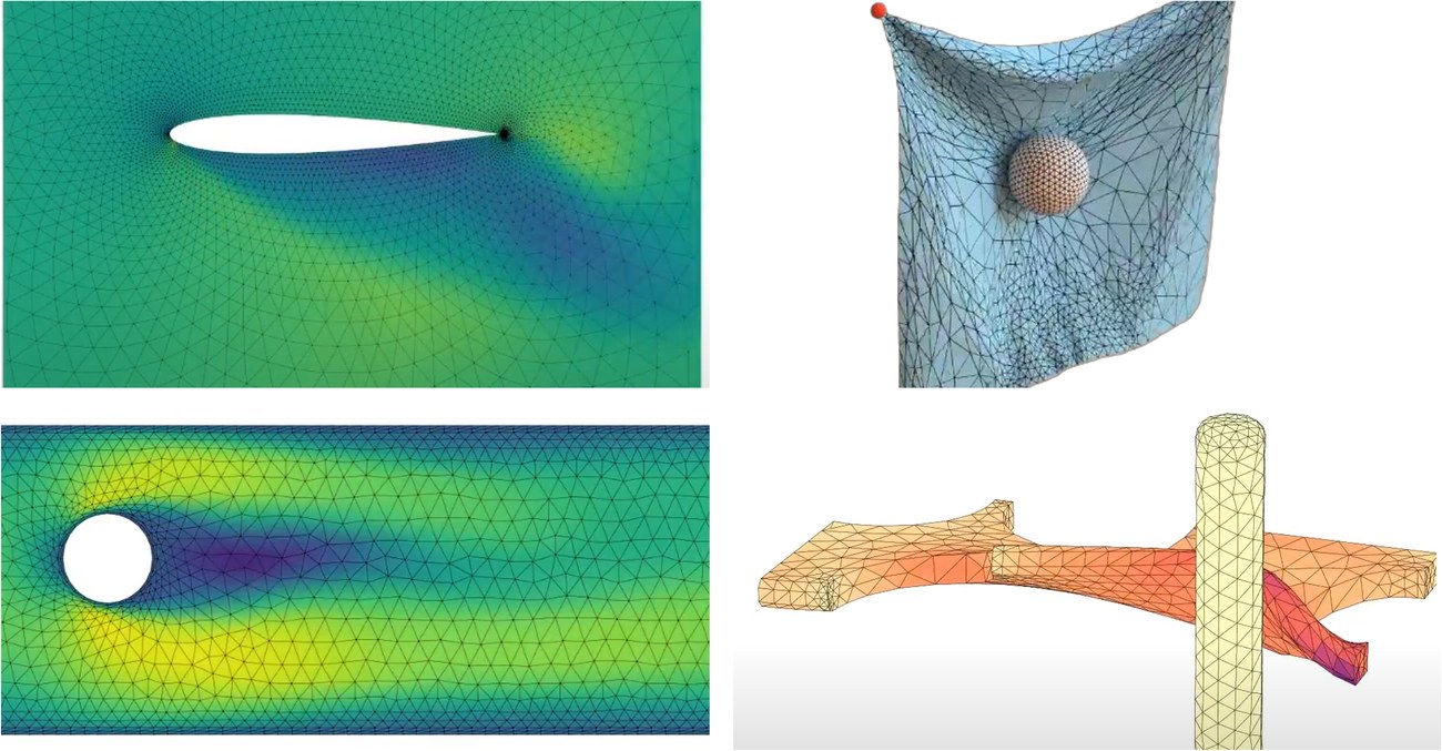
Applications

Forecasting dynamic systems

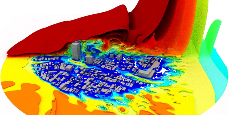
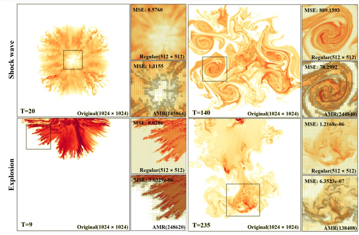
The central challenge is stability and mitigating error accumulation over long temporal rollouts, from planetary weather (FourCastNet) and urban microclimates to turbulence.

CityFFD urban microclimate data — The scale of the CityFFD dataset, as used by Peng et al. to model urban microclimates with FNOs.

Kolmogorov flow by the Markov neural operator — Kolmogorov flow simulated by the Markov neural operator from a Gaussian random field initial condition; the energy spectrum converges to the $k^{-5/3}$ cascade rate. Reproduced from Li et al.

AMR Transformer on adaptive meshes — Forecasting on adaptive meshes, with grid resolution varying across time-steps, is an open challenge. AMR-Transformer (Xu et al.) proposes a data-driven adaptive octree-based learning technique for this class of problems.

Heterogeneous and complex media

Here the difficulty is spatial heterogeneity: sharp discontinuities at multi-material interfaces and shocks, in porous media, inelastic impact and composite manufacturing.

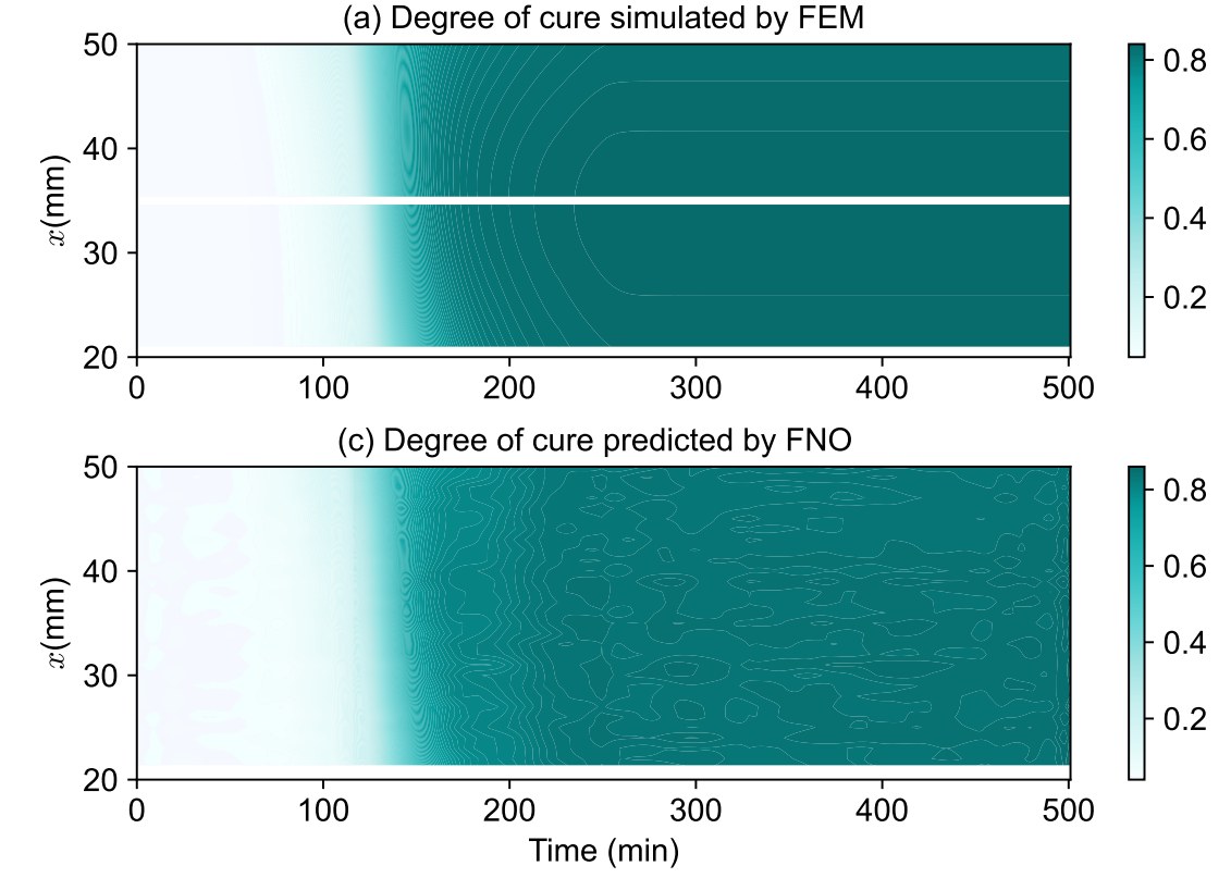
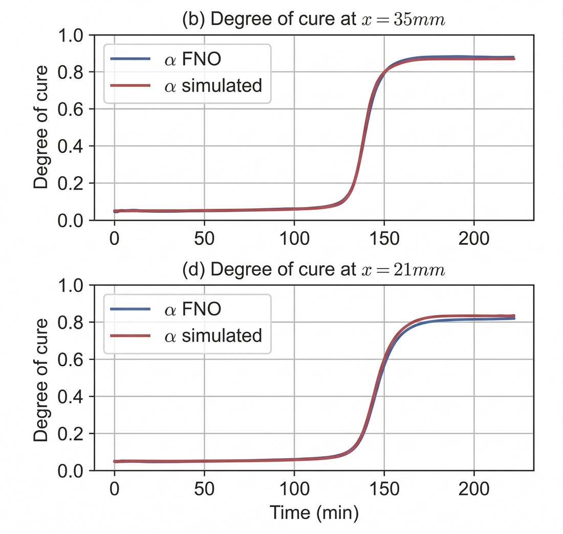
Degree of cure, FEM vs FNO — Degree of cure predicted by FEM vs. by FNO.

Degree of cure profiles — Degree of cure predicted by FNO and FEM at x = 35 mm and 21 mm.

Thermochemical curing of composites with residual FNOs (Chen et al.).

Inverse problems, design and optimization

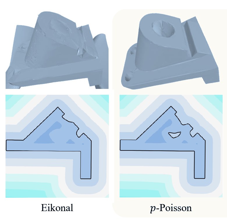
Operators are differentiable, which makes them natural surrogates for inverse problems and design, from bio-molecular design to physics-informed planning and surface reconstruction.

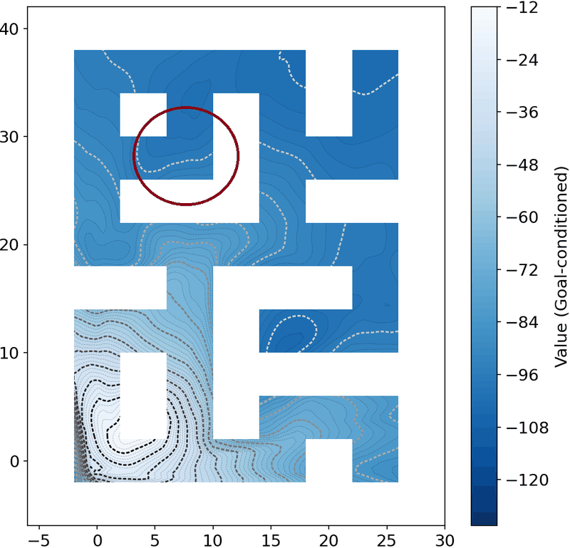
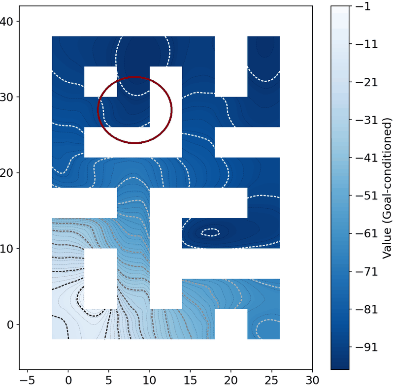
Value function, GCIVL with PINN — (b) GCIVL + PINN

Value function over a maze-like environment: PINN constraints improve its contours. Reproduced from Viswanath et al.

Level-set contours, Eikonal vs p-Poisson — Level-set contours from different physics-informed strategies (Eikonal vs. $p$-Poisson), as presented by Park et al.

Is Data All You Need?

"It is increasingly apparent that the future lies in synergy."

Neural operators trade a one-time training cost for very fast evaluation. In the survey's worked example, Bayesian inversion of Navier–Stokes with function-space MCMC, a conventional solver takes 2.2 s per evaluation and an FNO 0.005 s, after roughly 12 hours of training. For 100,000 evaluations on a cloud GPU instance, that is under $40 for the FNO, training included, against about $187 for the conventional solver. For a small number of evaluations, the conventional solver remains more efficient.

Numerical solvers are still needed to produce the training data, and the quality of that data bounds the operator. The survey's answer to its central question is therefore not replacement but complementarity: data-driven surrogates working in tandem with traditional solvers. It points to active learning, meta-learning and in-context learning to reduce data requirements, and to integrating operators into FEM software packages to make them accessible to physics researchers.

Code for the surveyed architectures

Citation

@article{viswanath2026neural,
  title   = {Neural Operator: Is data all you need to model the world? An insight into the paradigm of data-driven scientific ML},
  author  = {Viswanath, Hrishikesh and Rahman, Md Ashiqur and Vyas, Abhijeet and Shor, Andrey and Medeiros, Beatriz and
             Hernandez, Stephanie and Eswarappa Prameela, Suhas and Bera, Aniket},
  journal = {IEEE Transactions on Pattern Analysis and Machine Intelligence},
  year    = {2026}
}